Decision Tree

A decision tree is a tree-shaped diagram used to determine a course of action. Each branch of the tree represents a possible decision, occurrence, or reaction.

Example

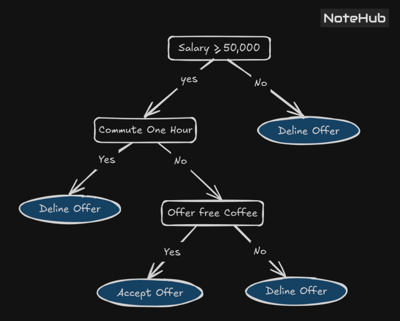
Consider a situation where someone is searching for a job. At the beginning of the process, they decide to consider only those jobs offering a monthly salary of at least ₹50,000. Additionally, they dislike spending excessive time commuting and are only comfortable if the travel time to work is less than an hour. They also expect the company to provide free coffee every morning.

The decision-making process regarding whether to accept or reject a job offer can be schematically represented using a decision tree.

This is a figure representing a decision tree:

Decision tree example showing classification based on salary, commute time, and incentives leading to accept or decline decision

Structure of a Decision Tree

A decision tree is a graph-theoretical tree, where:

Leaf nodes (represented as ellipses) indicate final decisions or outcomes.
Internal nodes (all nodes except the root) represent intermediate decisions based on various conditions.

Types of Decision Trees

Classification Trees: These are tree models where the target variable can take a discrete set of values. In a classification tree:
- Leaves represent class labels.
- Branches represent conjunctions of features leading to specific class labels.
Regression Trees: These trees handle target variables that take continuous values (i.e., real numbers). Examples include:
- Predicting the price of a house.
- Estimating the duration of a phone call.

Classification Tree,

See, we'll explain this with the help of an example.

A dataset is given to us, with features and class labels.

Advantages of Decision Tree

It is simple to understand, interpret, and visualize.
Little effort required for data preparation
Can handle both categorical and numerical data
Non-linear parameters do not affect its performance

Disadvantages of decision trees

Overfitting occurs when the A algorithm captures noise in the data.
High variance can cause the model to become unstable due to even slight variations in the data.
highly complicated decision tree tends to have low buyers, which makes it typical for the model to work with new data

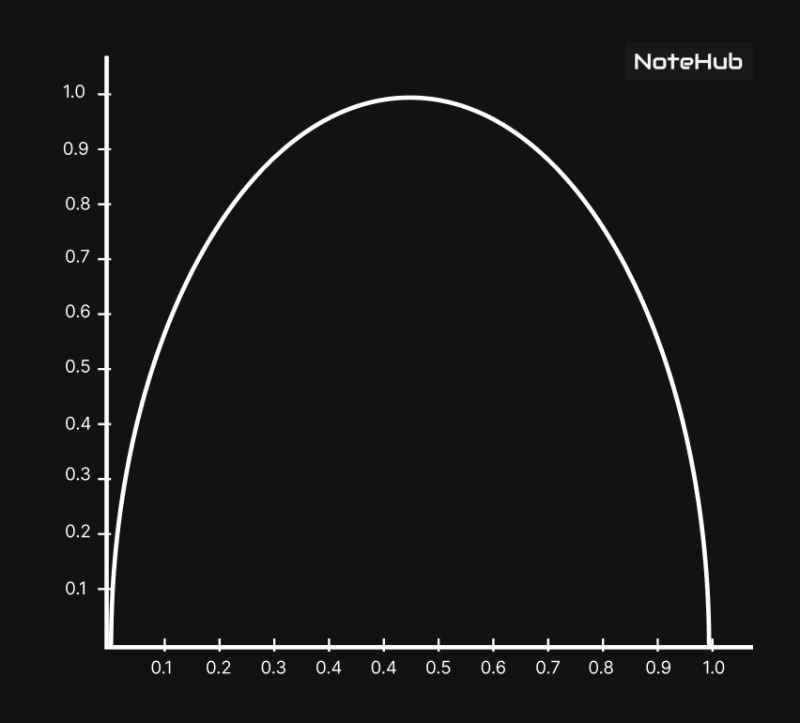
Entropy

entropy is a measure of impurity in a data set, sets with high entropy are very diverse and provide little information about other items that may also belongs in the set, as there is no apparent commonality entropy measured in bits, if there are only two possible classes, entropy value range from 0 to 1.
For classes, entropy ranges from 0 to . In each case, the minimum value indicates that the sample is completely homogenous, which the maximum value indicates that the data is as diverse as possible

Definition

consider a segment of dataset having number of class labels, let be the proportion of the examples m having the class label. then the Entropy of is defined as:

\text{Entropy}(S^{\prime})=-\sum_{i=1}^{c}p_{i}\log_2\left(p_{i}\right)

🔍 Where:

= the dataset (or subset of examples),
= number of classes (e.g., "Up", "Down"),
= proportion of examples in class ,
= logarithm base 2.

Decision tree visualization showing probability curve or decision boundary used to evaluate splits in classification

in this expression for Entropy, the value

💡 Example:

If you have:

4 "Up"
6 "Down"

Then:

p_{\text{Up}}=\frac{4}{10},\quad p_{\text{Down}}=\frac{6}{10}

Entropy=-\left(\frac{4}{10}\log_2\frac{4}{10}+\frac{6}{10}\log_2\frac{6}{10}\right)

That’s how you get the uncertainty of a dataset 🔥

Special Case

Let the data segment has only two class labels says "" and "" if is proportion of examples having class label "", then proportion of examples have label "", will be . in this case Entropy of is given by

Entropy\left(S^{\prime}\right)=-plog_2\left(p\right)-\left(1-p\right)log_2\left(1-p\right)

💡 Example:

Let be some class Label, then we denote the proportion of examples with class label i

S.no	Name	Give Birth	Aquatic Animal	Aerial Animal	Has Legs	Class Label
1	Human	Yes	No	No	Yes	Mammal
2	Python	No	No	No	No	Reptile
3	Salmon	No	Yes	No	No	Fish
4	Frog	No	Semi	No	Yes	Amphibian
5	Bat	Yes	No	Yes	Yes	Bird
6	Pigeon	No	No	Yes	Yes	Bird
7	Cat	Yes	No	No	Yes	Mammal
8	Shark	Yes	Yes	No	No	Fish

Let be the data in given table, the class label are

Class Label	Count
Mammal	2	2/8
Reptile	1	1/8
Fish	2	2/8
Amphibian	1	1/8
Bird	2	2/8

\text{Entropy}(S^{\prime})=-\sum_{\text{for all classes i}}p_{i}\log_2(p_{i})

-\left(\frac{2}{8}\log_2\frac{2}{8}\right)-\left(\frac{1}{8}\log_2\frac{1}{8}\right)-\left(\frac{2}{8}\log_2\frac{2}{8}\right)-\left(\frac{1}{8}\log_2\frac{1}{8}\right)-\left(\frac{2}{8}\log_2\frac{2}{8}\right)

= 0.5 + 0.375 + 0.5 + 0.375 + 0.5

=2.25

Information Gain:

Let be a set of Examples, A be a feature (or an attribute), be the subset of with , and value of be the set of all possible values of A. then the information gain of an attribute A relative to the set , denoted by

📘 Gain Formula:

\text{Gain}(S,A)=\text{Entropy}(S^{\prime})-\sum_{v\in\text{Values}(A)}\frac{|S_v|}{|S|}\cdot\text{Entropy}(S_{v})

🔍 Where:

= full dataset
= attribute (like Age, Type, etc.)
= all possible values of attribute A
= subset of S where attribute A has value v
= size of that subset
= size of total dataset
= entropy of that subset

Computation of

🔷 Attribute : gives birth(Yes, No)

Yes : = [Mammal, Mammal, Fish, Bird]

E=-\left(\frac{2}{4}\log_2\frac{2}{4}\right)-\left(\frac{1}{4}\log_2\frac{1}{4}\right)-\left(\frac{1}{4}\log_2\frac{1}{4}\right)

E=0.5+0.5+0.5

E=1.5

No : = [Reptile, Fish, Amphibian, Bird]

E=-\left(\frac{1}{4}\log_2\frac{1}{4}\right)-\left(\frac{1}{4}\log_2\frac{1}{4}\right)-\left(\frac{1}{4}\log_2\frac{1}{4}\right)-\left(\frac{1}{4}\log_2\frac{1}{4}\right)

E=0.5+0.5+0.5+0.5

E=2

=\text{Entropy}(S)-\frac{|S_{yes}|}{|S|}\cdot\text{Entropy}(S_{yes})\;-\frac{|S_{no}|}{|S|}\cdot\text{Entropy}(S_{no})\cdot\text{Entropy}(S_{no})

=2.25-\left(\frac{4}{8}\cdot1.5+\frac{4}{8}\cdot2\right)

2.25 - 1.75= 0.5

Gini Indices

The gini slit index of a dataset is another feature selection measure in the construction of classification tree. This measure is used in the cart algorithm.

Consider a data Set having Tau class labels let be the proportion of examples having the class label , The Gini index of the data set , denoted by Gini is defined by:

📘 Gain Formula:

Gini(S^{\prime})=1-\sum_{i=1}^{\tau}p_{i}^2

construct the decision tree using algorithm for given data set.

S.no	Age	Competition	Type	Profit (Class)
1	Old	Yes	Soft	Down
2	Old	No	Soft	Down
3	Old	No	Hard	Down
4	Mid	Yes	Soft	Down
5	Mid	Yes	Hard	Down
6	Mid	No	Hard	Up
7	Mid	No	Soft	Up
8	New	Yes	Soft	Up
9	New	No	Hard	Up
10	New	No	Soft	Up

🔧 Step 1: Initial Entropy of Dataset

Entropy(S^{\prime})=-p_{Up}log_2(p_{Up})-p_{Down}log_2(p_{Down})

Where:

Total = 10
Down = 5 (1 to 5)
Up = 5 (6 to 10)

So:

Entropy(S^{\prime})=-\frac{5}{10}\log_2\left(\frac{5}{10}\right)-\frac{5}{10}\log_2\left(\frac{5}{10}\right)

=-\frac{5}{10}log_2\left(\frac{1}{2}\right)-\frac{5}{10}log_2\left(\frac{1}{2}\right)

= -\frac{5}{10}log_2\left(2\right)^{-1} - \frac{5}{10}log_2\left(2\right)^{-1}

=\frac{5}{10}log_2\left(2\right)+\frac{5}{10}log_2\left(2\right)

=\frac{5}{10}\cdot1+\frac{5}{10}\cdot1

=0.5 + 0.5

✅ Entropy() = 1

Step 2: Calculate Information Gain for all attributes

Attribute 1: Age (Old, Mid, New)

Old : = [Down, Down, Down]

E=-\frac{3}{3}\log_2\frac33

E = 0

Mid : = [Down, Down, Up, Up]

=-\frac{2}{4}log_2\frac{2}{4}-\frac{2}{4}log_2\frac24

$$$

New : = [Up, Up, Up]

E=-\frac{3}{3}log_2\frac33

=\text{Entropy}(S^{\prime})-\frac{|S_{old}|}{|S|}\cdot\text{Entropy}(S_{old})-\frac{|S_{mid}|}{|S|}\cdot\text{Entropy}(S_{mid})-\frac{|S_{new}|}{|S|}\cdot\text{Entropy}(S_{new})

=1-\left(\frac{3}{10}\cdot0+\frac{4}{10}\cdot1+\frac{3}{10}\cdot0\right)

1 - 0.4 = 0.6

✅ Gain(Age) = 0.6

Attribute 2: Competition (Yes, No)

Yes : = [Down, Down, Down, Up]

=-\frac{3}{4}log_2\frac{3}{4}-\frac{1}{4}log_2\frac14

E=-0.75\cdot\log_20.75-0.25\cdot\log_20.25

E \approx 0.811

No : = [Down, Down, Up, Up, Up, Up]

=-\frac{2}{6}log_2\frac{2}{6}-\frac{4}{6}log_2\frac46

E=-0.333.\log_20.333-0.666.\log_20.666

E \approx 0.918

=1-\left(\frac{4}{10}\cdot0.811+\frac{6}{10}\cdot0.918\right)

\approx1-(0.3244+0.5508)=0.1248

✅ Gain(Competition) = 0.125

Attribute 3: Type (Soft, Hard)

Soft : = [Down, Down, Down, Up, Up, Up]

E=-\frac{3}{6}log_2\frac{3}{6}-\frac{3}{6}log_2\frac{3}{6}

E=-\frac12\log_2\frac12-\frac12\log_2\frac12

E = -0.5\log_{2}2^{-1} -0.5\log_{2}2^{-1}

E=0.5\cdot1+0.5\cdot1

E=1

Hard : = [Down, Down, Up, Up]

E=-\frac{2}{4}log_2\frac{2}{4}-\frac{2}{4}log_2\frac{2}{4}

E=-\frac{1}{2}\log_2\frac{1}{2}-\frac{1}{2}\log_2\frac12

E = -0.5\log_{2}2^{-1} -0.5\log_{2}2^{-1}

E=0.5\cdot1+0.5\cdot1

E=1

=1-\left(\frac{6}{10}\cdot1+\frac{4}{10}\cdot1\right)

=1-(0.6+0.4)=0

✅ Gain(Type) = 0

Find the maximum Gain

✅ Gain(Age) = 0.6

✅ Gain(Competition) = 0.125

✅ Gain(Type) = 0

\text{max}\left(0.6,0.125,0\right)=0.6

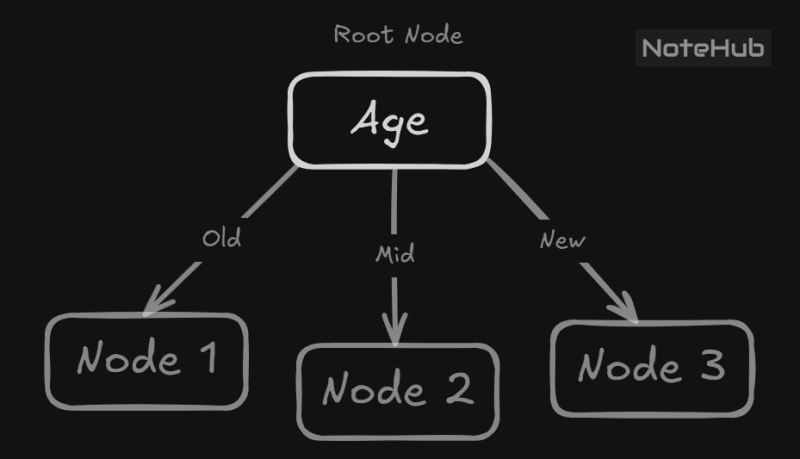
Age gives the highest gain (0.6).

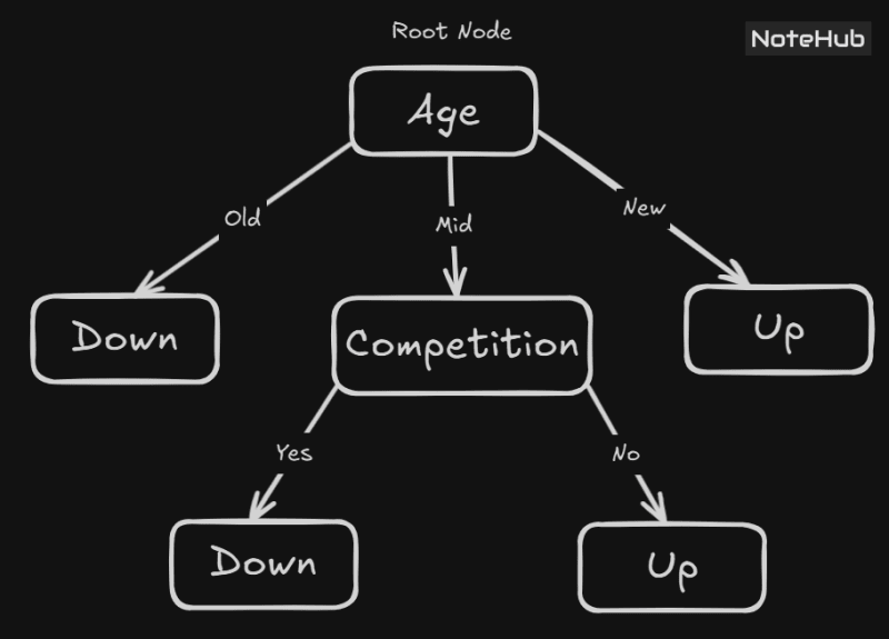
Thus, "Age" will be placed at the root of Decision Tree.

The Decision Tree Formation

Decision tree diagram with root node “Age” splitting into branches (Old, Mid, New) leading to child nodes

, a subset of for which Age = Old

Age	Competition	Type	Profit (Class)
Old	Yes	Soft	Down
Old	No	Soft	Down
Old	No	Hard	Down

Observation:

All 3 examples → Profit = Down
✅ Pure group!

thus

Entropy(S^1)=0

Leaf Node = "Down"

a subset of for which Age = Mid

Age	Competition	Type	Profit (Class)
Mid	Yes	Soft	Down
Mid	Yes	Hard	Down
Mid	No	Hard	Up
Mid	No	Soft	Up

Observation:

2 examples → Down
2 examples → Up

Entropy\left(S^2\right)=-\frac{2}{4}log_2\frac{2}{4}-\frac{2}{4}log_2\frac24

Entropy\left(S^2\right)=1

✅ Mid group is impure (entropy = 1).
Further splitting needed.

🔷Attribute 1: Competition(Yes, No)

Yes : = [Down, Down]

Entropy(\text{Yes})=0

No: = [Up, Up]

Entropy(\text{No})=0

=1-\left(\frac{2}{4}\cdot0+\frac{2}{4}\cdot0\right)

1-0=1

✅ Gain(Competition) = 1

🔷Attribute 2: Type(Soft, Hard)

Soft: = [Down, Up]

-\frac{1}{2}log_2\frac{1}{2}-\frac{1}{2}log_2\frac12\;=\;1

Hard : = [Down, Up]

-\frac{1}{2}log_2\frac{1}{2}-\frac{1}{2}log_2\frac{1}{2}\;=\;1

=1-\left(\frac{2}{4}\cdot1+\frac{2}{4}\cdot1\right)

1-1=0

✅ Gain(Type) = 1

Since the Gain is maximum for the attribute, so putting the competition at Node 2

a subset of for which Age = New

Age	Competition	Type	Profit (Class)
New	Yes	Soft	Up
New	No	Hard	Up
New	No	Soft	Up

All 3 examples → Profit = Up
✅ Pure group!

Entropy(New)=0

Leaf Node = "Up"

Decision tree with root “Age” and secondary split “Competition,” leading to final outcomes Down or Up.

All the corresponding class labels are down in
✅ Pure group!

Entropy(New)=0

Leaf Node = "Down"

All the corresponding class labels are up in
✅ Pure group!

Entropy(New)=0

Leaf Node = "Up"